Heewon Hwang

In a burgeoning field of machine learning (ML) in finance, a paper published by Shihao Gu, Bryan Kelly, and Dacheng Xiu (GKX, 2021) introduces a novel asset pricing model that leverages autoencoder neural networks. The underlying idea of the paper is elaborate yet intuitive, as it takes the next logical step in the evolution of asset pricing models.

Background: Evolution of Empirical Asset Pricing

Asset pricing ultimately deals with the question of why different assets are priced differently and earn different returns. The theoretical framework devised to tackle this matter was to use the notion of risk compensation–different assets have different “risk factors” and their returns can be derived from the compensation investors would receive for taking such risks.

From this logic, the most basic asset pricing model could be set up as follows:

\[r_{i,t} = \beta_{i,t} f_{t} + \epsilon_{i,t}\]

• $r_{i,t}$ : return of asset $i$ at time $t$
• $\beta_{i,t}$ : loading of factor $f$ for asset $i$ at time $t$
• $f_t$ : factor value (return) at time $t$
• $\epsilon_{i,t}$ : error term (noise) for asset $i$ at time $t$

Using this fundamental model, empirical analysis developed in two contrasting approaches: the “classical”, known factors approach and the “Bayesian-like”, latent factors approach.

Known Factors Approach

This approach is more classical to finance literature, having its roots in the Capital Asset Pricing Model (CAPM) and Fama-French Three Factor Model. Its core idea is using pre-determined factors derived from what is already “known” about asset returns to estimate the factor loadings (betas) through regression. For instance, Eugene Fama and Kenneth French famously observed that (1) small firms tend to outperform big firms in stock returns and (2) stocks with high book-to-market values tend to outperform those with low book-to-market values. They then utilized firm size and book-to-market value (along with market excess return) as the explanatory risk factors in their Three Factor Model.

Now, as with any other regression problem, the known factors approach is limited by the fact that some degree of understanding or insight about asset returns is required beforehand. Like an endless loop, researchers must already know something about asset returns in order to extract meaningful factors that will help them know something asset returns.

Furthermore, since the initial knowledge or intuition that is readily available is likely imperfect, it could lead to the formation of factors that aren’t informative. Finding just the right combination of factors to include in the model while leaving all irrelevant factors out (model setting) is yet another issue.

Latent Factors Approach

Using latent factors addresses the limitations of the known factors approach by employing a Bayesian-like approach. Its core idea is to remove the prerequisite of established knowledge and “let the data speak for itself”. It treats all relevant factors as latent (existing but not yet discovered) and statistically extracts factors purely from data. A famous technique used with latent factors is Principal Component Analysis (PCA), which extracts the principal components of a large variable set (factors in our case) by capturing the direction of maximum variance in the data.

This approach, however, is limited in that (1) its factor loadings are static and (2) it can only use returns data. It fails to take advantage of utilizing other relevant information that could be used as conditional data to improve the model’s performance. Quite the opposite of the known factors approach, using latent factors has its limitations of not being able to utilize what is already known.

Kelly, Pruitt, and Su (KPS, 2019)

KPS, which can be thought of as the predecessor study to GKX, created a novel approach of Instrumented Principal Component Analysis (IPCA) by taking the pros and leaving the cons of the above two approaches. While it maintains the overall design of the latent factor approach, it allows for the factor loadings (betas) to depend on observable characteristics ($z_{i,t-1}$) of stocks through linear mapping:

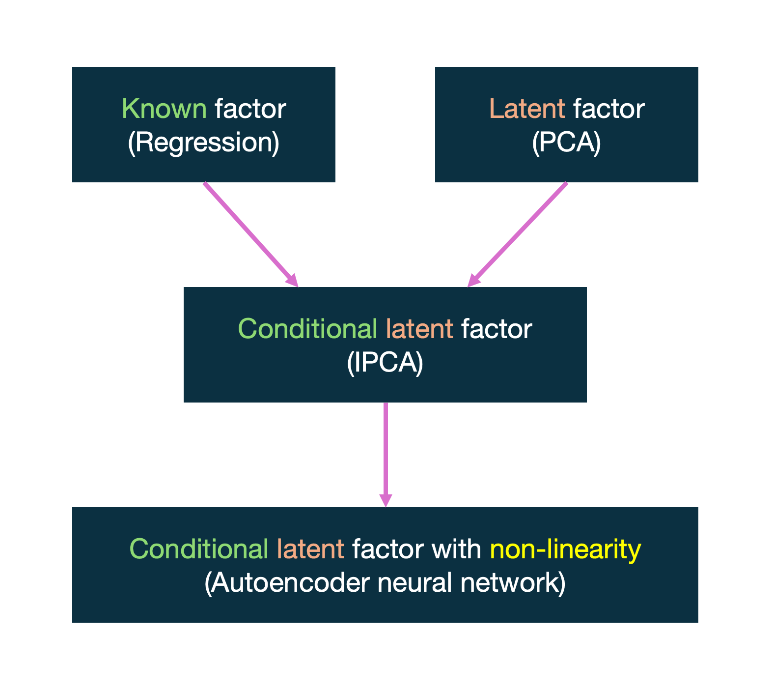
\[r_{i,t} = \beta(z_{i,t-1}) f_t + \epsilon_{i,t},\] \[\beta(z_{i,t-1}) = z_{i,t-1} \Gamma\]

This allows the model to not be overly reliant on established knowledge (like the known factor approach) but also not completely dismiss it (like the latent factor approach) by appropriately incorporating it as proxies for conditional and time-varying factor loadings. It effectively presents a conditional latent factor approach that can utilize known factors for conditional factor loadings.

KPS specifically used asset-specific covariates such as size, value, and momentum in estimating factor loadings, which not only improved the factor loading estimate but also improved the estimation of latent factors themselves.

While IPCA is a notable improvement to empirical methodology in asset pricing, it is still bounded by the linearity restriction of PCA which allows for the simplification of reality, but fails to capture its complexities. And this is where GKX comes in. GKX generalizes the IPCA model by allowing for non-linearity with the use of autoencoder neural networks.

Below figure summarizes the background for the study:

Why Autoencoder Makes Sense

About Autoencoders

Autoencoder is a type of neural network that is primarily used for unsupervised learning tasks, such as dimensionality reduction and feature extraction. A simple autoencoder with a single hidden layer is shown below:

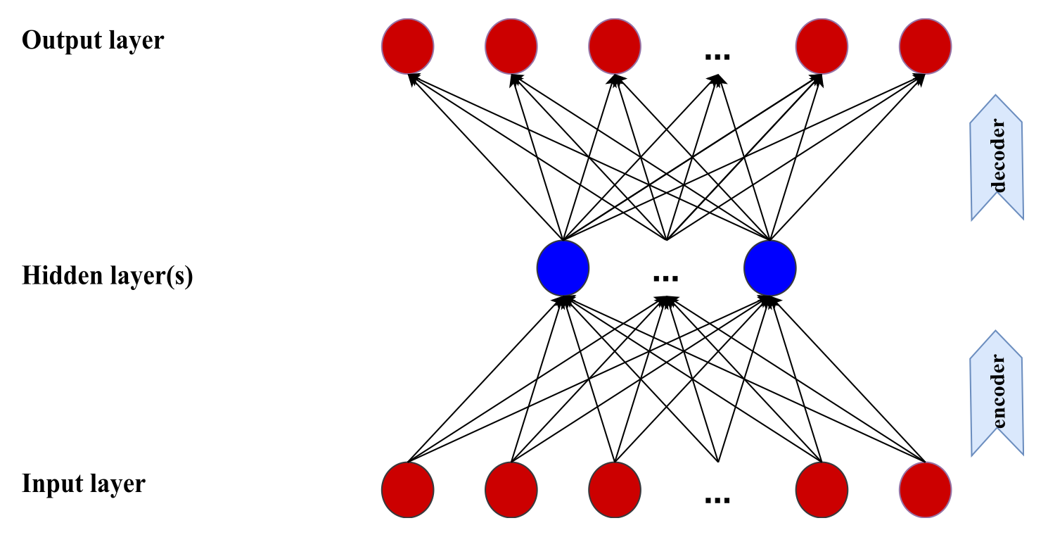
The autoencoder consists of 2 primary components: encoder and decoder. The encoder takes input data and compresses it into a lower dimensional representation in the hidden layer (also called the bottleneck). Since dimensionality is to be reduced, the hidden layer contains fewer neurons than the input layer. After the encoding process, the decoder aims to reconstruct the original input data from its lower dimensional representation. The decoding result is stored in the output layer having the same dimensions as the input layer.

In our context of extracting informative latent factors from asset returns, the hidden layer would contain such factors as compressed representation of asset returns.

A mathematical representation of what goes on inside autoencoders can be outlined as below. The equation is a recursive formula describing a vector of outputs from layer $l$ $(l>0)$ :

\[r^{(l)} = g \left( b^{(l-1)} + W^{(l-1)} r^{(l-1)} \right)\]

• $N$ : number of inputs
• $L$ : number of layers
• $l$ : given layer
• $r_k^{(l)}$ : output of neuron $k$ in layer $l$
• $r^{(l)} = (r_1^{(l)}, …, r_k^{(l)})$ : vector of outputs from layer $l$
• $r^{(0)} = (r_1, …, r_N)$ : input layer (= cross section of $N$ asset returns)
• $g(\cdot)$ : activation function (GKX uses ReLU $\rightarrow$ $g(y) = \text{max}(y, 0)$)
• $b^{(l-1)}$ : $K^{(l)} \times 1$ vector of bias parameters from layer $l-1$
• $W^{(l-1)}$ : $K^{(l)} \times K^{(l-1)}$ matrix of weight parameters from layer $l-1$

The underlying function of an autoencoder is similar to any other neural network. After the input layer is fed, a recursive process of linear combination of bias, weight parameters, and previous layer’s output that undergoes an activation function is passed forward.

What is unique in autoencoders is in the optimization process. Instead of minimizing the error between the output and an external solution, the difference between the output and input are set to be minimized.

Implementing Autoencoder Factor Models

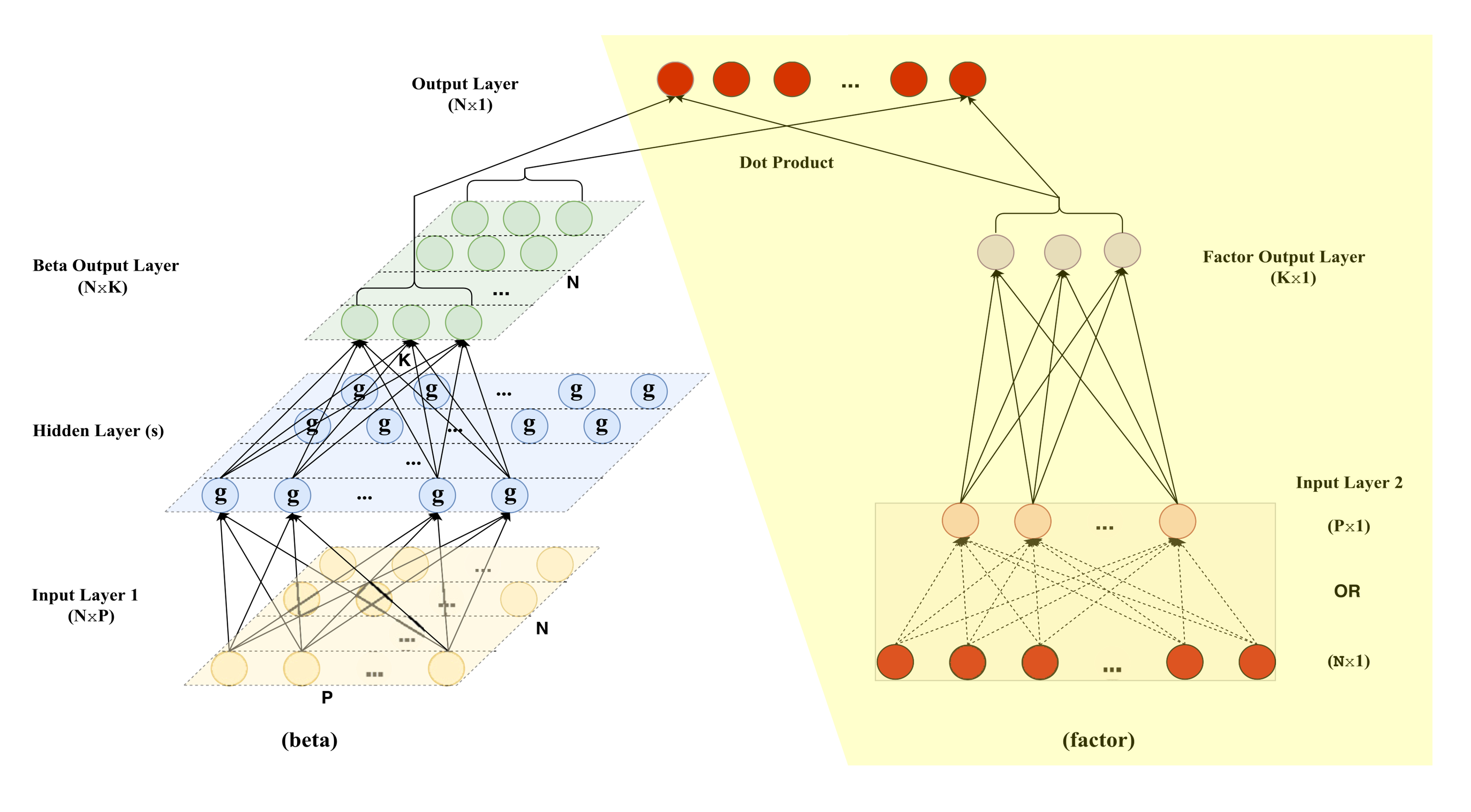
A simple autoencoder as illustrated above has the same limitation as PCA as it doesn’t utilize conditioned factor loadings. Like PCA, it only uses asset returns as input data to extract factors and doesn’t really bother with factor loadings. Hence, like the IPCA, a way to embed conditional estimates of factor loadings is needed, and GKX accomplishes this by adding a separate neural network alongside the autoencoder that specializes in factor loading estimations.

This is well illustrated in the figure provided below:

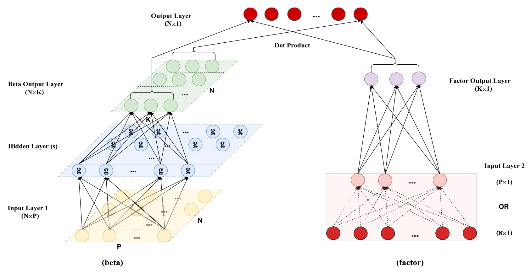
The neural network on the left is the newly introduced network that is tasked with conditional factor loading estimations.

Note: unlike how an autoencoder was used to extract factors, the new network is an ordinary neural network and not an autoencoder. This is evident as the input layer of the network has different dimensions from the output layer.

The network conducts conditional factor loading estimates by using the “known” asset characteristics as input, performing the usual forward propagation, and outputing factor loadings as a $N \times K$ matrix of betas.

The neural network on the right side, then, must be the autoencoder that has and will be used for factor estimation. Yet, a modification is made to the autoencoder’s input layer for practical and interesting reasons.

Note: it must be noted that the autoencoder technically encompasses the following portion of the overall model:

As also shown in the illustration, the input layer undergoes a clustering process whereby asset returns are grouped into portfolio returns. GKX explains the modification stating the following reasons

1. To reduce the number if weight parameters that need to be calculated
2. To account for unbalanced/incomplete stock returns data (monthly availability of stock returns may vary widely)
3. To allow for conditional factor estimation (through grouping portfolios by certain asset characteristics)

While the first two reasons are for practicality, the third reason yields an interesting consideration. Through grouping assets by meaningful asset characteristic portfolios, it allows for conditional factor estimations to occur without the need for attaching an external dataset of asset characteristics to the autoencoder as the portfolio returns will have information of asset characteristics embedded within them. Interestingly, this turns a once conditional problem with static asset returns into a static problem with conditional portfolio returns.

A minor modification was also made to the autoencoder’s final output layer, where it is now calculated as a dot product between the conditional factor loading estimates (green matrix) and the hidden layer of the autoencoder (layer with purple neurons). This is to incorporate the conditional factor loading estimates into the overall optimization process.

Below is a mathematical representation of the workings of the new model.

First, recall from the beginning that the most basic asset pricing model can be represented as follows:

\[r_{i,t} = \beta_{i,t} f_{t} + \epsilon_{i,t}\]

The left neural network of the model used for conditional factor loading estimates can be mathematically depicted as follows:

\[z_{i,t-1}^{(0)} = z_{i,t-1},\] \[z_{i,t-1}^{(l)} = g \left( b^{(l-1)} + W^{(l-1)} z_{i,t-1}^{(l-1)} \right), \quad l = 1, \dots, L_\beta,\] \[\beta_{i,t-1} = b^{(L_\beta)} + W^{(L_\beta)} z_{i,t-1}^{(L_\beta)}\]

Altogether, it is a recursive computation of conditional factor loadings ($\beta_{i,t-1}$) using lagged asset characteristics ($z_{i,t-1}$) as inputs. The asset characteristics are lagged as their data is not readily available; data update intervals range from monthly, quarterly, to annual releases.

The right autoencoder of the model used for factor estimates can be mathematically shown as follows:

\[r_{t}^{(0)} = r_{t},\] \[r_{t}^{(l)} = \tilde{g} \left( \tilde{b}^{(l-1)} + \tilde{W}^{(l-1)} r_{t}^{(l-1)} \right), \quad l = 1, \dots, L_f,\] \[f_{t} = \tilde{b}^{(L_f)} + \tilde{W}^{(L_f)} r_{t}^{(L_f)}\]

Together, the equations show a recursive computation of factor estimates ($f_t$) using a standard autoencoder.

If the activation function were to be linear, the following optimization task would need to be solved to train the hyperparameters:

\[\min \sum_{t=1}^{T} \left\| r_t - \beta_{i,t} f_t \right\|^2 = \min_{W_0, W_1} \sum_{t=1}^{T} \left\| r_t - Z_{t-1} W_0 W_1 x_t \right\|^2\]

• $Z_t = (z_{1,t}, z_{2,t}, \dots, z_{N,t})’$ : input layer of asset characteristics (yellow layer of left network)
• $\beta_{i,t} = Z_{t-1} W_0$ : conditional factor loadings estimates (green layer of left network)
• $x_t = \left( Z_{t-1}’ Z_{t-1} \right)^{-1} Z_{t-1} r_t$ : input layer of portfolio returns (layer of pink neurons of right autoencoder)
• $f_t = W_1 x_t$ : factor estimates (layer of purple neurons of right autoencoder)

Note: in testing the model, non-linear activation function (ReLU) was used

For additional reference, below are methods employed by GKX to prevent overfitting issues of the model:

• Training, validation, testing
  • Split data into 3: training, validation, testing
  • Validation sample was used to “tune” hyperparameters, intended to simulate an out-of-sample (OS) performance before doing an actual OS test with testing data
• Regularization technique
  • LASSO (L1 regularization)
  • early stopping (L2 regularization)
  • ensemble approach in training (using multiple random seeds for initial weights and calculating the final estimate as the average of results)
• Optimization algorithms
  • adaptive moment estimation (Adam) algorithm
  • batch normalization

Results

GKX tested the autoencoder asset pricing model with US stock data. Specifications of the data used are below:

• Monthly individual US stock returns from three major exchanges (NYSE, AMEX, NASDAQ)
  • Doesn’t filter returns based on stock prices or share code, and doesn’t rule out financial firms (usually done to exclude outliers)
• T-bill as proxy for risk-free rate
• Data range from March 1957 ~ Dec 2016 (60 years)
• 94 stock-level characteristics based on previous asset pricing literature
• Data split
  • Training: 18 yrs (1957 ~ 1974)
  • Validation: 12 yrs (1975 ~ 1986)
  • OS testing: 30 yrs (1987 ~ 2016)

The specifications of conditional autoencoder (CA) models used are as follows:

• CA0: single linear layer (no hidden layer) in both factor and factor loading (beta) networks
• CA1: single linear layer for factor, 1st hidden layer with 32 neurons for factor loading
• CA2: single linear layer for factor, 2nd hidden layer with 16 neurons for factor loading
• CA3: single linear layer for factor, 3rd hidden layer with 8 neurons for factor loading

To evaluate the performance of CA models in context, the following models were used as comparisons:

• Fama-French factor models (FF) with 1 ~ 6 factors (classical model of known factors)
• PCA
• IPCA

Statistical Performance

The statistical performance of models were assessed on two different $R^2$ metrics:

\[R^2_{\text{total}} = 1 - \frac{\sum_{(i,t) \in \text{OOS}} (r_{i,t} - \hat{\beta}'_{i,t-1} \hat{f}_t)^2}{\sum_{(i,t) \in \text{OOS}} r_{i,t}^2}\]

• Tests how well the model can explain the variation in returns across stocks by using “contemporaneous” factor loadings ($\hat{\beta}’_{i,t-1}$) and factor realizations ($\hat{f}_t$)

\[R^2_{\text{pred}} = 1 - \frac{\sum_{(i,t) \in \text{OOS}} (r_{i,t} - \hat{\beta}'_{i,t-1} \hat{\lambda}_{t-1})^2}{\sum_{(i,t) \in \text{OOS}} r_{i,t}^2}\]

• Evaluates the predictive power of the model by examining how well it can predict future stock returns by using lagged average of factors up to time $t-1$ ($\hat{\lambda}_{t-1}$) instead of factors for each time period

$R^2_{\text{total}}$ results are shown as below:

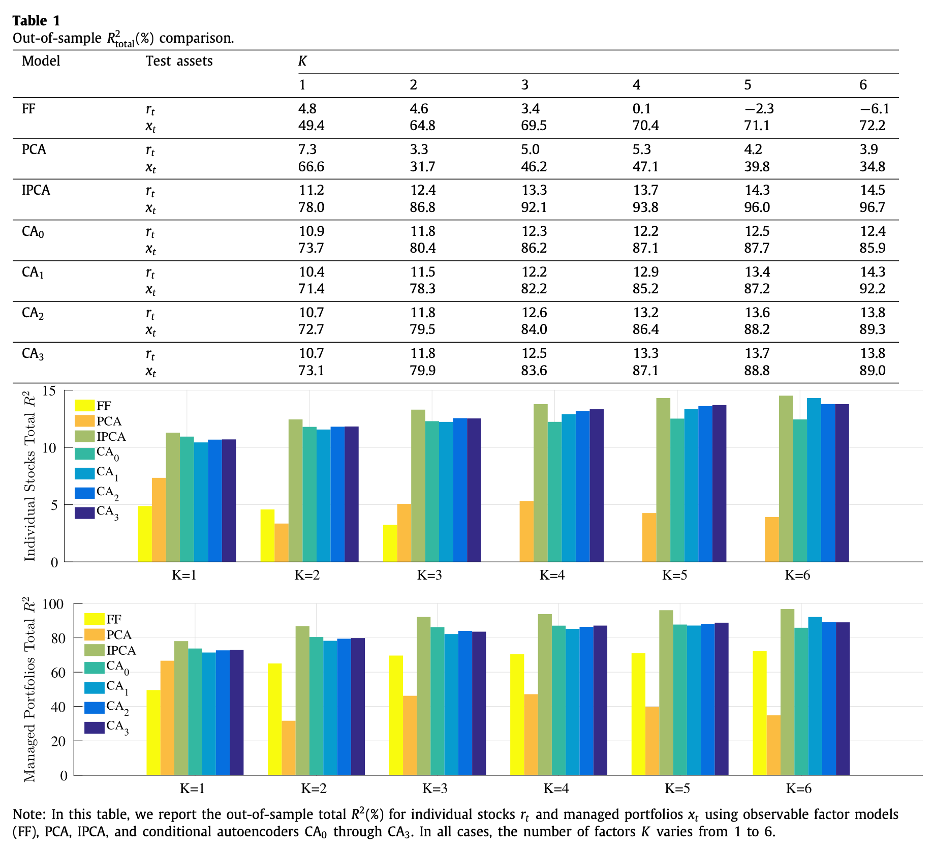
From using individual stock returns as input, the performance of static models (FF, PCA) are poor whereas the conditional models (IPCA, CA0~3) show strong performance. When using managed portfolio returns, performance of FF greatly increase but still underperforms the conditional models

$R^2_{\text{pred}}$ results are shown as below:

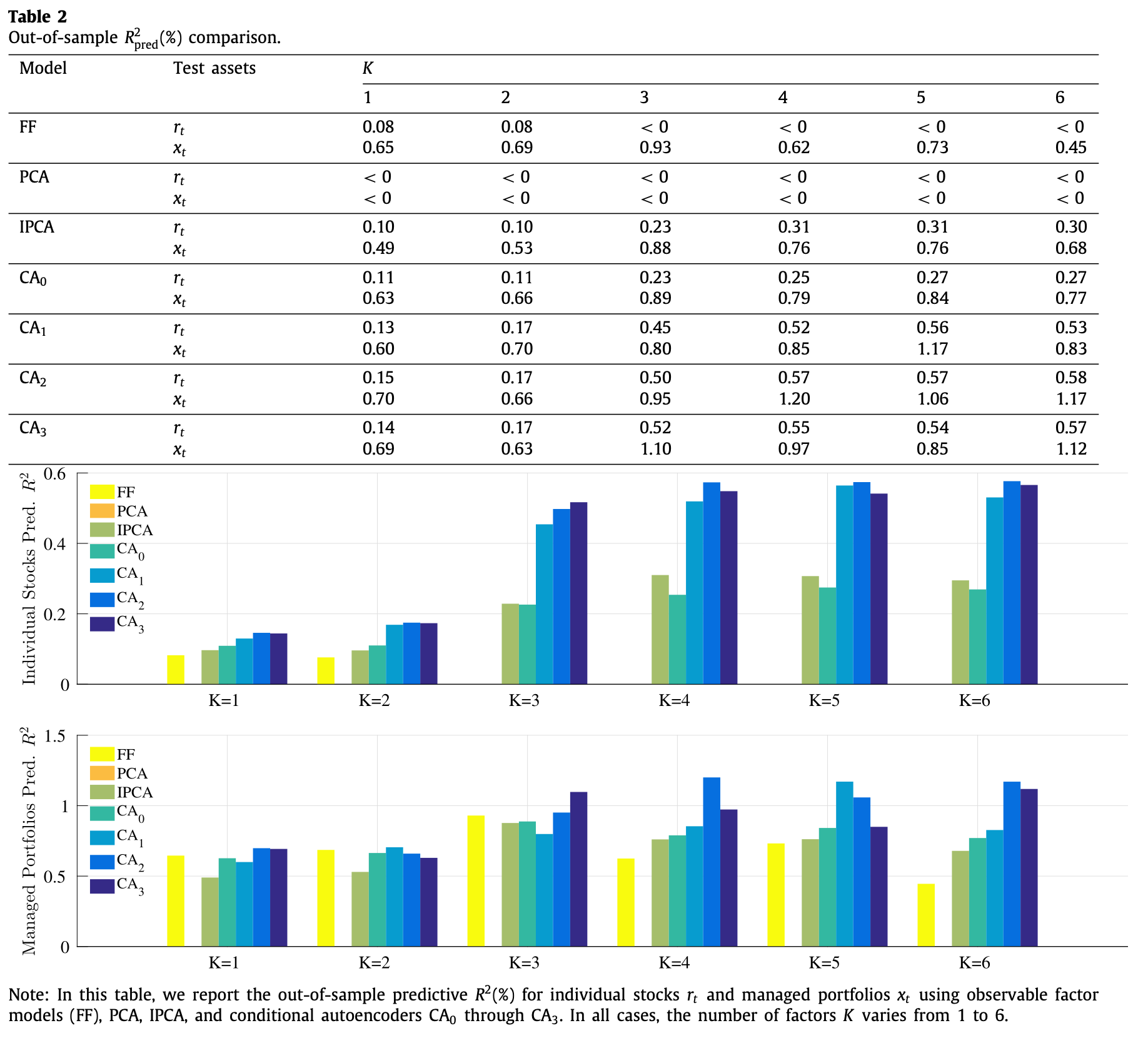
This is the more interesting result. While with $R^2_{\text{total}}$ IPCA performed superbly, if not better than the CA models, its dominance is greatly subdued here. The performance of CA models are dominant across the board, but it is interesting to note that when based on managed portfolios, the dominance is less pronounced.

Economic Performance

To see if the CA models work in investing contexts, GKX conducted a comparison of models’ Sharpe ratios. The ratios were calculated from investment portfolios that buys the highest expected return stocks (decile 10) and sells the lowest expected return stocks (decile 1) based on each model’s sorting of stocks by their OS return forecasts. The portfolios were rebalanced monthly, and two versions, equal weighted and value weighted, were simulated.

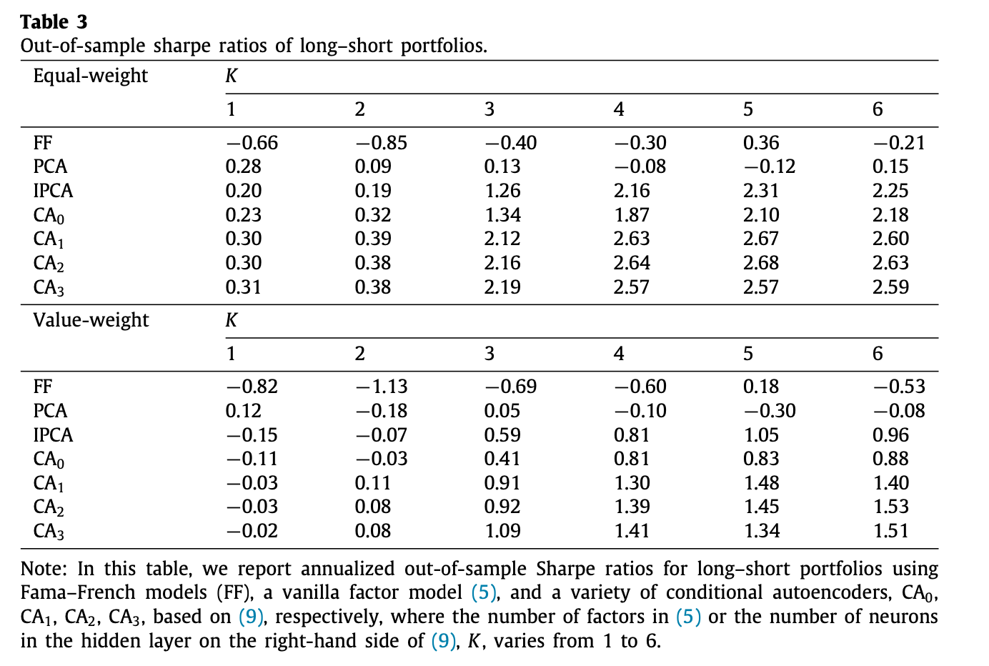
The results are similar to those from $R^2_{\text{pred}}$ where the overall magnitude of Sharpe ratios are ranked as: CA2 > CA1, CA3 > IPCA > PCA > FF

Characteristic Importance

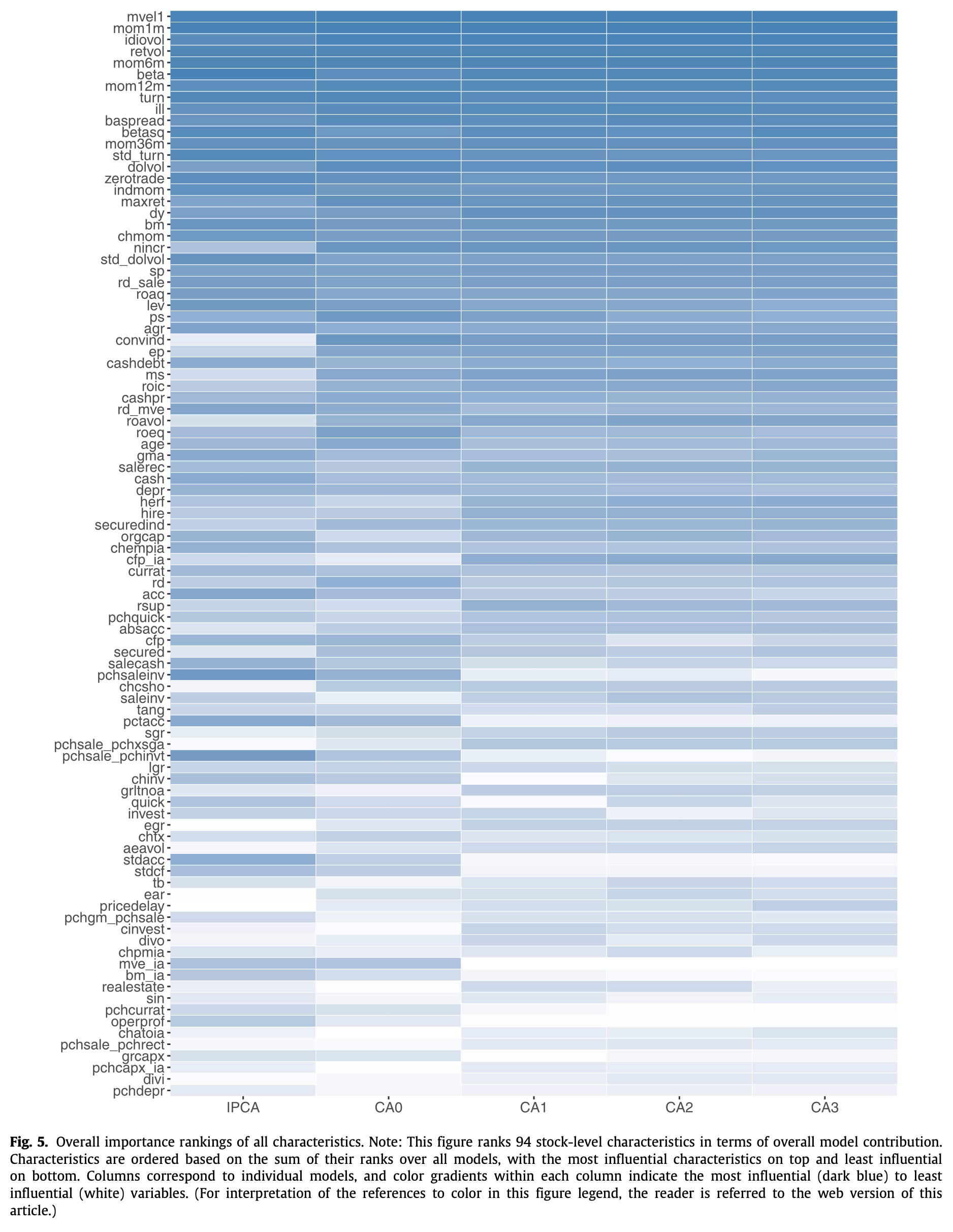
Using the CA models, GKX also looked at the relative importance of asset characteristics calculated from their impact on the $R^2$ metrics. The top 20 characteristics in each CA model were ranked as follows

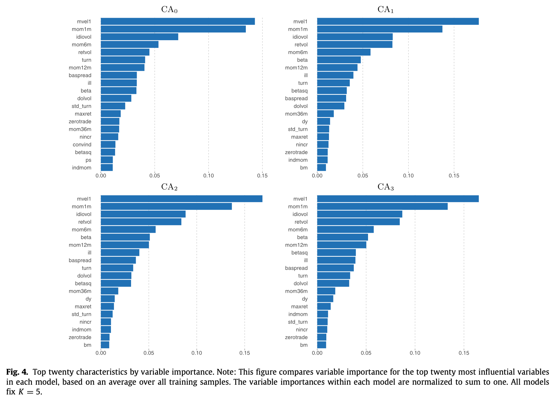
It was noted that the top 20 characteristics were really what mattered–top 20 accounted for 80% of explanatory power in CA0 and 90% in CA1~3. Also, all CA variants pointed to the same 3 strongest characteristic categories: price trend, liquidity, and risk measures.

• price trend
  • short-term reversal (mom1m), stock momentum (mom12m), momentum change (chmom), industry momentum (indmom), recent maximum return (maxret), and long-term reversal (mom36m)
• liquidity
  • turnover and turnover volatility (turn, std_turn), log market equity (mvel1), dollar volume (dolvol), Amihud illiquidity (ill), number of zero trading days (zerotrade), and bid–ask spread (baspread)
• risk measures
  • total and idiosyncratic return volatility (retvol, idiovol), market beta (beta), and beta- squared (betasq)

The full ranking is as follows:

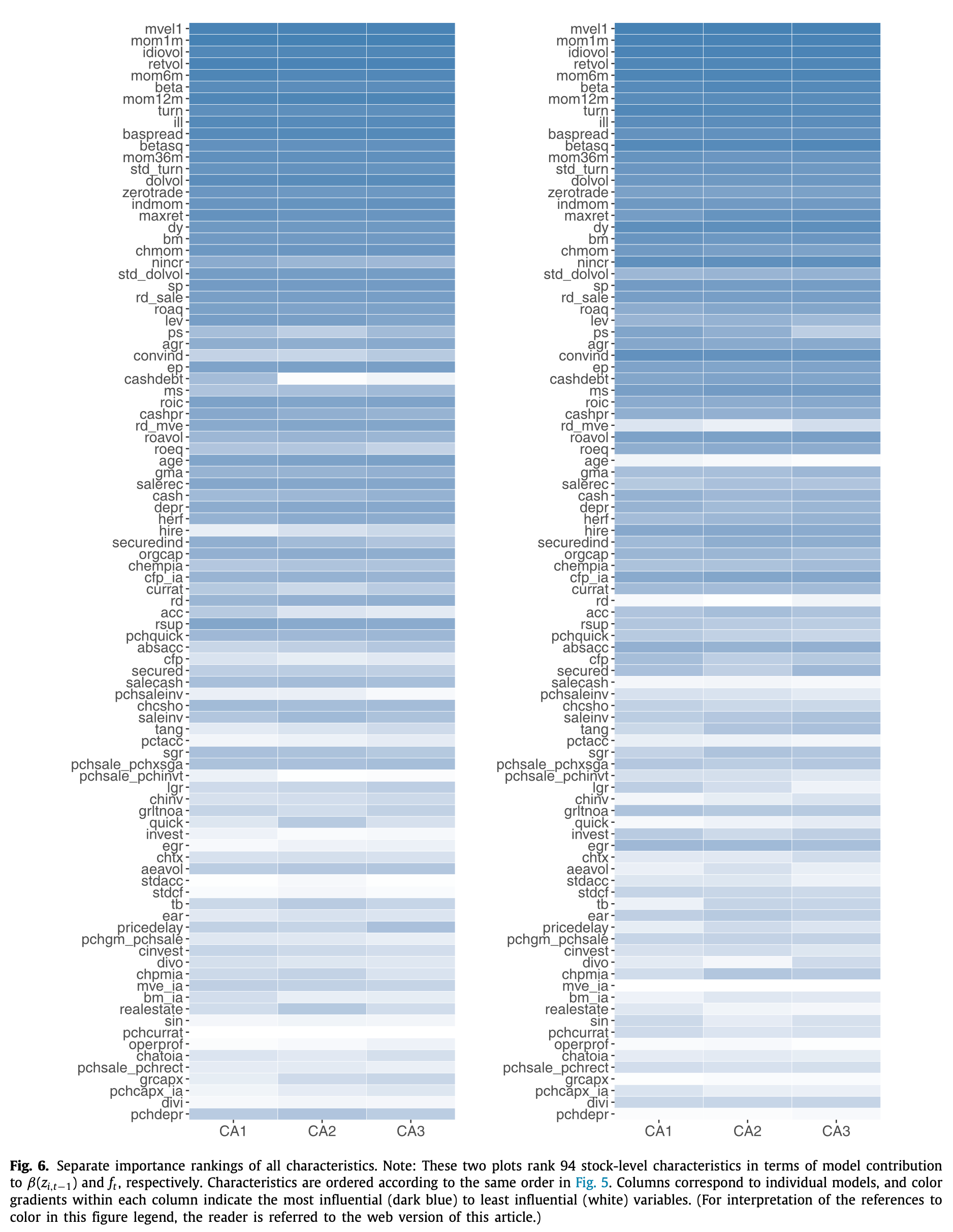
GKX also separately ranked the characteristic importance in factor loading estimation (left) and factor estimation (right) networks but found similar results.

Thoughts

I believe GKX provides a very interesting novel asset pricing model that well employs ML techniques in order to address the limitations of previous asset pricing methodology. While dealing with non-linear models in finance can be dangerous due to the low signal-to-noise ratio in financial data and thus the greater likelihood of overfitting, it can be seen that GKX imposed numerous cautionary measures to account for such risks.

I do, however, hold some questions, especially regarding the use of data.

Firstly, the data split seemed a bit unorthodox as of the 60 years of data available, only 30% (18 years) of it was used for training. Typically, more data is used for training than in testing to provide a more robust model, but GKX did the opposite. Hence, it could raise concerns about whether sufficient model training was done. Furthermore, in addition to the amount of training data used, its quality can be brought into question. GKX trained their model using the oldest data they had available, using returns data from 1950s to 1970s. This is concerning not only because older financial data is generally of less quality with lower credibility but more so because of the wide temporal gap between the financial market that the model was trained on and the market it was asked to understand and predict. Market conditions constantly change over time, and what was once considered important factors in the 1950s and 1970s may be less important in 2000s and 2010s.

Secondly, I had to wonder if the the overall data was enough to begin with. while the cross-sectional data seemed more than enough (considering the dropping of data filters), the time-series data was collected monthly for a total range of 60 years. This would yield a maximum of 720 datapoints per stock or portfolio along the time-series which could be considered insufficient especially for training neural networks.

Lastly, I would like to point out an area of further research that could branch off from the work of GKX. I found the characteristic importance findings to be very interesting and think insights from them could be re-applied to the autoencoder model. For istance, it could be used for practical purposes: since only 20 of the 94 asset characteristics were realistically important, we could cut down on the asset characteristic input data for the factor loading neural network to only include the important 20 characteristics. This could speed up the training and re-fitting process of the model. It might also be interesting to see the performance of classical, known factor model fitted with the top 20 asset characteristics as its factors. It could greatly improve the model’s performance but could also have adverse affects as the correlational relationship between the asset characteristics is yet to be known.

References

1. Gu S., Kelly B., Xiu D. (2021) Autoencoder asset pricing models. J. Econometrics 222 (1), 429–450.
2. Kelly, B., Pruitt, S., Su, Y. (2019) Characteristics are covariances: A unified model of risk and return. J. Financ. Econ. 134 (3), 501–524.
3. IBM Technology YouTube Video about Autoencoders